3. Data Quality Assurance

Data quality assurance is at the core of GGIR. GGIR undertakes several key tasks aimed at evaluating, where possible enhancing the quality of the data, and documenting how data was enhanced. These tasks include time gap identification and imputation, automatic calibration of the sensors, identification of periods when sensors were not worn , and scrutiny for segments of the signal exhibiting sustained, unusually high accelerations that are rarely encountered in real-world scenarios.

Time gaps identification and imputation

The time gap identification and imputation functionality offered by GGIR is exclusive to ActiGraph gt3x files, Axivity cwa files, and ad-hoc csv files. This is because there are potential time gaps in these file formats. GGIR has been developed to efficiently identify and manage these time gaps.

Time gaps in Axivity cwa files

Although this is not expected to occur often, Axivity cwa data can come with faulty data blocks. In Axivity cwa files, a data block represents a few seconds of data. For example, faulty blocks may occur when the device is connected to a computer with a USB cable. To address this, R package GGIRread, which is used by GGIR to read cwa files, identifies these faulty blocks and imputes them by the last recorded non-faulty acceleration value normalised to 1 g.

Axivity devices are expected by design to have a slightly variable sampling rate, which is accounted for by resampling the data. The interpolation technique used for resampling is set by parameter interpolationType, and uses linear interpolation by default (interpolationType = 1) but you can also set it to nearest neighbour interpolation (interpolationType = 2). As a quality assurance, GGIRread keeps track of the variation in sampling rate per data block and automatically imputes blocks where the sampling rate deviates by more than 10% from the expected sampling rate. If you are unhappy with this threshold then note that you can change this percentage with parameter frequency_tol. Biased sampling rates of this kind are expected to be extremely rare, but we nonetheless like to be able to account for them.

Additionally, to monitor this process, GGIRread logs a series of file health statistics which are stored by GGIR in the ‘data_quality_report.csv’ file located within the ‘QC’ folder of the output directory ‘results’. Within this file, variable names prefixed with ‘filehealth’, detailing the number and duration of time gaps detected during recording, as well as number of epochs with 5-10% and more than 10% biases in the sampling rate.

Time gaps in ActiGraph gt3x and ad-hoc csv files

Some manufacturers incorporate functionalities in their devices to let them stop recording during long episode of no movement, aiming to conserve battery life and reduce data size. However, this feature results in recorded signals containing intermittent time gaps that must be accounted for during data processing.

For example, ActiGraph has the option called idle sleep mode in their devices, which makes data collection pause when there is no movement for a sustained period of time. The ActiGraph’s idle sleep mode is explained in the manufacturer’s website.

GGIR imputes gaps shorter than 90 minutes at raw data level, using the last known recorded value normalised to 1 g. While gaps longer than 90 minutes are imputed at epoch level to make the data processing more memory efficient and faster. These time gaps in the data are considered non-wear time in GGIR, this implies that we trust the accelerometer to only cause timegaps when it is not worn, although there is always a risk of sleep/sedentary misclassification. GGIR logs the number and duration of the time gaps found in the ‘data_quality_report.csv’ file located within the ‘QC’ folder of the output directory ‘results’.

Studies often forget to clarify whether the accelerometers were configured to pause data collection during periods of no movement and, if so, how the resulting time gaps were accounted for in the data processing. Especially, if the device firmware or manufacturer software already imputes the time gaps that can cause significant bias to the GGIR estimates. More generally speaking, we advise:

• Disable such functionality if possible as it harms the transparency and reproducibility since no mechanism exists to replicate the time gaps in other accelerometer brands, and it is likely to challenge accurate assessment of sleep and sedentary behaviour.

• That data collected with ‘idle sleep mode’ or similar functionalities is not referred to as raw data accelerometry, because the data collection process has involved proprietary pre-processing steps which violate the core principle of raw data collection.

• Report whether ‘idle sleep mode’ or similar functionalities were used.

Specific note on ActiGraph idle sleep mode

ActiGraph files might be exported in gt3x or csv formats. When idle sleep mode is used then the data in these files are different. In gt3x files, time gaps can be found in the signal, with no imputation made by the ActiLife software. However, csv files exported in ActiLife will have imputed values in all three axes during periods of no movement. Note that this imputation by the ActiLife software has changed at some point in time. Initially the imputation was zeros but with more recent versions of ActiLife the imputation uses the last recorded value for each axis. Therefore, you need to be aware that GGIR will take care of the time gap imputation relative to the idle sleep mode when using gt3x files, but not when using ActiGraph csv files (because the latter come with the time gaps already imputed).

Auto-calibration algorithm

An acceleration sensor works on the principle that acceleration is captured mechanically and converted into an electrical signal. The relationship between the electrical signal and the acceleration is usually assumed to be linear, involving an offset and a gain factor. We shall refer to the establishment of the offset and gain factor as the sensor calibration procedure. Accelerometers are usually calibrated as part of the manufacturing process under non-movement conditions using the local gravitational acceleration as a reference. The manufacturer calibration can later be evaluated by holding each sensor axis parallel (up and down) or perpendicular to the direction of gravity; readings for each axis should be ±1 and 0 g, respectively. However, this procedure can be cumbersome in studies with a high throughput. Furthermore, such a calibration check will not be possible for data that have been collected in the past and for which the corresponding accelerometer device does not exist anymore. Techniques have been proposed that can check and correct for calibration error based on the collected triaxial accelerometer data in the participant’s daily life without additional experiments, referred to as autocalibration.

The general principle of these techniques is that a recording of acceleration is screened for non-movement periods. Next, the rolling average over the nonmovement periods is taken from each of the three orthogonal sensor axes and used to generate a three-dimensional ellipsoid representation that should ideally be a sphere with radius 1 g. Here, deviations between the radius of the three-dimensional ellipsoid and 1 g (ideal calibration) can then be used to derive correction factors for sensor axis-specific calibration error. This auto-calibration performed by GGIR uses this technique and a more detailed description and demonstration can be found in the published paper.

The success of the auto-calibration depends on the number of no-movement periods and variation of accelerometer orientation during those periods available to the algorithm. As a result, auto-calibration is expected to perform less in very short recordings (e.g., less than a day ) or in recordings in which the participant did not wear the accelerometer for most of the time. In such cases, you can use other recordings from the same sensor that have more no-movement periods in a higher variation of orientations to derive its calibration coefficients, and then apply these coefficients to the recording of interest. To do so, you should use the parameter backup.cal.coef, see specific documentation on this parameter [here](https://cran.r-project.org/package=GGIR/vignettes/GGIRParameters.html#:~:text=setting%20is%20TRUE.-,backup.cal.coef,-Character%20(default%20%3D%20%E2%80%9Cretrieve).

The auto-calibration algorithm is applied by default but can be turned off with the parameter do.cal = FALSE. We do not recommend turning off the autocalibration unless you have strong reasons to do so.

Non-wear detection

Accelerometer non-wear time is detected on the basis of statistics derived from a rolling time window over the raw data. A time interval is classified as non-wear if both of the following criteria are met for at least two out of the three accelerometer axes:

• The standard deviation of the accelerations is less than accelerometer brand specific reference values, which for most brands is 13.0 mg (\(1 mg = 0.00981 m·s^−2\))
• The range of accelerations (i.e., maximum value minus minimum value) is less than 50 mg.

The size of the rolling time window and the size of the steps it takes in time are defined by parameter windowsizes, a vector with length three. More specifically, the first value is used as epoch size for acceleration metric calculation and not used for non-wear detection, the second value is the resolution of the classification ( default = 15 min) and the third value is the window size use for classification (default = 60 min) are used.

How it then labels the data depends on how parameter nonwear_approach is specified. At the moment there are two options: nonwear_approach = "2013" and nonwear_approach = "2023" (default). This initial detection and labelling of non-wear periods occurs in GGIR part 1.

Approaches to detect non-wear: 2013 and 2023 algorithms

nonwear_approach = “2013”

The 2013 approach is a revision of an approach first described in a 2011 PLoSONE publication. It applies the criteria discussed above to a rolling 60-minute window to classify the 15 minute window in its centre . This means that the windows overlap by 22.5 minutes.

nonwear_approach = “2023”

The 2023 version of the algorithm uses the criteria applied to the 60-minute window to assign a non-wear score to that entire window. Instead of centring the 60 minute window in the middle of the 15 minute window, the 60 minute window’s left edge is aligned to the left edge of the 15 minute window. As a result, each 15-minute window is classified multiple times given that multiple steps of the rolling window classification will overlap with it. If the non-wear criteria are met for any of these windows that overlap with the 15-minute window, it will be labelled as non-wear.

Relabelling implausible wear as non-wear

Inspection of non-wear classifications indicated that the algorithm as described above does not cope well with periods of monitor transportation per post. Here, long periods of non-wear are briefly interrupted by periods of movement, which are interpreted by the algorithm as monitor wear. Therefore, in GGIR part 2, the detected non-wear from part 1 is screened for implausible wear periods which are then relabelled as non-wear. All detected wear-periods of less than six hours and less than 30% of the combined duration of their bordering non-wear periods ar e relabelled as non-wear. Additionally, all wear-periods of less than three hours and which form less than 80% of their bordering non-wear periods are classified as non-wear. 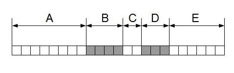The motivation for selecting a relatively high criterion (< 30%) in combination with a long period (6 hrs) and a low criterion (< 80%) in combination with a short period (3 hrs) is that long periods are more likely to be actually related to monitor wear time. To illustrate the algorithm we created a visual model, see picture below. Here, units of time are presented in squares and marked grey if detected as non-wear time. Period C is detected as wear-time and borders to non-wear periods B and D. If the length of C is less than six hours and C divided by the sum of B and D is less than 0.3 then the first criteria is met and block C is turned into a non-wear period.

Visual inspection of >100 traces from a large observational study revealed that applying this stage three times iteratively allowed for improved classification of periods characterised by intermittent periods of non-wear and apparent wear.

Relabelling the wear in the beginning and end of the recording

The final 24 hours are often considered the period in which the accelerometer is potentially taken off but moved because of transportation, e.g., by the mail service. All wear-periods in the final 24 hrs of each measurement shorter than three hours and preceded by at least one hour of non-wear time are classified as non-wear.

Finally, if the measurement starts or ends with a period of less than three hours of wear followed or preceded by non-wear (any length) then this period of wear is classified as non-wear. These additional criteria for screening the beginning and end of the accelerometer file reflect the likelihood of movements that are involved when starting the accelerometer or downloading the data from the accelerometer. This final check can be turned off with parameter nonWearEdgeCorrection, which may be relevant when processing accelerometer data collected during single night polysomnography studies.

Clipping detection

GGIR part 1 also screens the acceleration signal for “clipping”, i.e., sustained unusual high (raw) acceleration values non compatible with human movement. If more than 30% of the data points in a 15-minute window (same as used for non-wear) are close to the maximal values (technical term for this is dynamic range) of this sensor the corresponding time period is considered as potentially unreliable, which may be explained by the sensor getting stuck at its extreme value or accelerometers being used inappropriately (attached to some heavily accelerating object). For example, for a dynamic range of 8g, accelerations over 7.5g would be marked as “clipping”. The window is also classified as clipping if any value in the window is larger than 150% the dynamic range of the sensor. Given that clipping rarely happens it is reported by GGIR as part of non-wear time. They are treated the same and by merging them we arrive at a single indicator for the amount of valid data. However, to keep track of the occurrence of clipping time GGIR does report the fraction of 15-minute windows during which clipping occurs, see section on output below.

Key parameters

Time gap imputation

• imputeTimegaps

Auto-calibration

• do.cal
• backup.cal.coef

Non-wear detection

• windowsizes
• nonwear_approach
• nonWearEdgeCorrection

Clipping detection

• windowsizes
• dynrange

GGIR output

(Part of) variable name	Description	Report(s)
calib_err	Calibration error (static estimate) Estimated based on all ‘non-movement’ periods in the measurement after applying the autocalibration	part2_summary.csv
calib_status	Calibration status: Summary statement about the status of the calibration error minimisation	part2_summary.csv
calib_status	Calibration status: Summary statement about the status of the calibration error minimisation	part2_summary.csv
N hours	Number of hours of measurement in a day, which typically is 24, unless it is a day on which the clock changes (DST) resulting in 23 or 25 hours. The value can be less than 23 if the measurement started or ended this day	part2_summary.csv and part2_daysummary.csv
N valid hours	Number of hours with valid data in the day	part2_summary.csv and part2_daysummary.csv
fraction_night_invalid	Fraction of the night (noon-noon or 6pm-6pm) for which the data was invalid, e.g. monitor not worn or no accelerometer measurement started/ended within the night	part4_nightsummary and part4_summary_sleep
nonwear_perc_day	Non-wear percentage during the waking hours of this day	part5_daysummary and part5_summary
nonwear_perc_spt	Non-wear percentage during the sleep period time hours of this day	part5_daysummary and part5_summary
nonwear_perc_day_spt	Non-wear percentage during the whole day, including waking and sleep period time	part5_daysummary and part5_summary
clipping_score	The Clipping score: Fraction of 15 minute windows per file for which the acceleration in one of the three axis was close to the maximum for at least 80% of the time. This should be 0	part2_summary.csv
cal.error.start	Calibration error (static estimate) Estimated based on all ‘non-movement’ periods in the measurement before applying the autocalibration	QC/data_quality_report.csv
cal.error.end	Calibration error (static estimate) Estimated based on all ‘non-movement’ periods in the measurement after applying the autocalibration	QC/data_quality_report.csv
QCmessage	Calibration status: Summary statement about the status of the calibration error minimisation	QC/data_quality_report.csv
NFilePagesSkipped	(Only for Axivity .cwa format) Number of raw data blocks skipped	QC/data_quality_report.csv
filehealth_totimp_min	(Only for Axivity .cwa, ActiGraph gt3x, and ad-hoc csv format) Total number of minutes of raw data imputed	QC/data_quality_report.csv
filehealth_checksumfail_min	(Only for Axivity .cwa format) Total number of minutes of raw data where the checksum failed	QC/data_quality_report.csv
filehealth_niblockid_min	(Only for Axivity .cwa format) Total number of minutes of raw data with non-incremental block ids	QC/data_quality_report.csv
filehealth_fbias0510_min	(Only for Axivity .cwa format) Total number of minutes with a sampling frequency bias between 5 and 10%	QC/data_quality_report.csv
filehealth_fbias1020_min	(Only for Axivity .cwa format) Total number of minutes with a sampling frequency bias between 10 and 20%	QC/data_quality_report.csv
filehealth_fbias2030_min	(Only for Axivity .cwa format) Total number of minutes with a sampling frequency bias between 20 and 30%	QC/data_quality_report.csv
filehealth_fbias30_min	(Only for Axivity .cwa format) Total number of minutes with a sampling frequency bias higher than 30%	QC/data_quality_report.csv
filehealth_totimp_N	(Only for Axivity .cwa, ActiGraph gt3x, and ad-hoc csv format) Total number of data blocks that were imputed	QC/data_quality_report.csv
filehealth_checksumfail_N	(Only for Axivity .cwa format) Total number of blocks where the checksum failed	QC/data_quality_report.csv
filehealth_niblockid_N	(Only for Axivity .cwa format) Total number of raw data blocks with non-incremental block ids	QC/data_quality_report.csv
filehealth_fbias0510_N	(Only for Axivity .cwa format) Total number of raw data blocks with a sampling frequency bias between 5 and 10%	QC/data_quality_report.csv
filehealth_fbias1020_N	(Only for Axivity .cwa format) Total number of raw data blocks with a sampling frequency bias between 10 and 20%	QC/data_quality_report.csv
filehealth_fbias2030_N	(Only for Axivity .cwa format) Total number of raw data blocks with a sampling frequency bias between 20 and 30%	QC/data_quality_report.csv
filehealth_fbias30_N	(Only for Axivity .cwa format) Total number of raw data blocks with a sampling frequency bias higher than 30%	QC/data_quality_report.csv

References

• van Hees VT, Fang Z, Langford J, Assah F, Mohammad A, da Silva IC, Trenell MI, White T, Wareham NJ, Brage S. Autocalibration of accelerometer data for free-living physical activity assessment using local gravity and temperature: an evaluation on four continents. J Appl Physiol (1985). 2014 Oct 1;117(7):738-44. PMID: 25103964 link

• van Hees VT, Gorzelniak L, Dean León EC, Eder M, Pias M, Taherian S, Ekelund U, Renström F, Franks PW, Horsch A, Brage S. Separating movement and gravity components in an acceleration signal and implications for the assessment of human daily physical activity. PLoS One. 2013 Apr 23